Covariance, Correlation, and Regression
How two assets move together, and how to read the line that summarizes it.
Retrieve before reading
In one sentence: a portfolio holds 50% SPY and 50% IWM. Which number from lesson 0000 - the mean or the standard deviation - needs information about how the two funds move together?
Reveal a strong answer
The standard deviation. The portfolio's expected return is a weighted average (linearity of expectation, P5 in lesson 0000). Its variance is not - it depends on how the two assets co-move. That co-movement is this lesson.
Why co-movement is the whole game
Lesson 0000 showed \(\text{Var}(aX) = a^2\text{Var}(X)\). Now take two assets. The variance of a sum is not the sum of variances:
The extra term is the covariance, defined as
Read it in plain terms: take each pair of deviations from the means, multiply them, and average. When both assets surprise in the same direction, the product is positive; when they surprise oppositely, it is negative. Covariance is the expected product of two surprises.
Mastery derivation 1: the two-asset portfolio variance
This derivation is a unit mastery target (MISSION.md). We derive it from the definition of variance - no formula sheet.
Let a portfolio hold weight \(w\) in asset 1 and \(1-w\) in asset 2, so \(r_p = w r_1 + (1-w) r_2\). We want \(\text{Var}(r_p)\).
Step 1. Write variance as the expected squared deviation from the mean:
Step 2. By linearity of expectation, \(E[r_p] = w E[r_1] + (1-w) E[r_2]\). Subtract this from \(r_p\):
Step 3. Square. Let \(d_i = r_i - E[r_i]\) to keep the algebra readable:
Step 4. Take expectations. The expectation of \(d_i^2\) is \(\text{Var}(r_i)\) by definition. The expectation of \(d_1 d_2\) is \(\text{Cov}(r_1, r_2)\) by definition. Therefore:
That is the two-asset portfolio variance, derived from nothing but the definition of variance and linearity of expectation. The term \(2w(1-w)\text{Cov}\) is the entire reason diversification works: if the covariance is low or negative, the combined risk is smaller than either asset alone.
For \(n\) assets the pattern generalizes: \(\sigma_p^2 = \sum_i\sum_j w_i w_j \text{Cov}(r_i, r_j)\). Each pair of assets contributes its covariance weighted by both weights. Unit 3 (0013) uses this matrix form to derive the frontier; lesson 0012 uses it to show why portfolio risk falls toward the average covariance as \(n\) grows.
Correlation: covariance, normalized
Covariance has units (percent-squared) and an unbounded size, which makes it hard to judge. Dividing by the two standard deviations fixes both problems:
Correlation always lies in \([-1, 1]\).
- \(\rho = 1\): perfectly co-moving; the assets are the same risk in disguise. No diversification.
- \(\rho = -1\): perfectly opposite; some combination eliminates risk entirely.
- \(\rho = 0\): uncorrelated (not necessarily independent); the covariance term vanishes, so the weighted variance terms simply add. Risk does not disappear, but it does not compound.
Rewriting the two-asset formula with correlation:
Everything that matters about co-movement is in \(\rho\).
Diversification is a statement about correlation, not about the number of assets. Holding 50 stocks that all move with the market does not diversify market risk; it only cancels each stock's own noise. The frontier of Unit 3 is exactly this trade-off drawn out.
Mastery derivation 2: the OLS slope
The second unit mastery target: where does beta come from? From a regression line fit by least squares. Given observations \((x_t, y_t)\), the line \(\hat{y} = a + bx\) is chosen to minimize the sum of squared residuals \(\sum_t (y_t - a - b x_t)^2\). We derive \(b\).
Step 1. Minimize over \(a\) first. Set the derivative with respect to \(a\) to zero:
So \(\sum_t (y_t - a - b x_t) = 0\), which says the residuals sum to zero, i.e. \(\bar{y} = a + b\bar{x}\). The fitted line passes through the means; call this the intercept condition.
Step 2. Use the intercept condition to eliminate \(a\). Since \(a = \bar{y} - b\bar{x}\), the residual is
Write centered variables \(\tilde{y}_t = y_t - \bar{y}\), \(\tilde{x}_t = x_t - \bar{x}\). The objective is now \(\sum_t (\tilde{y}_t - b\tilde{x}_t)^2\).
Step 3. Minimize over \(b\):
Step 4. Solve:
That is the least-squares slope: the covariance of \(x\) and \(y\) divided by the variance of \(x\). In returns language, regressing an asset's returns on the market's returns gives exactly
where \(r_m\) denotes the market return. This is the beta of the index model (Unit 4) and the CAPM's risk measure (0017). Note what the derivation shows: beta is not a magic number from a vendor; it is the slope of the best-fitting line through the paired returns.
Real market artifact: two funds, one line
Below are the 119 monthly returns of SPY (S&P 500 ETF) and IWM (Russell 2000 small-cap ETF), 2016-08-20 to 2026-08-20, fetched live from Yahoo Finance. The artifact: compute the moments, then teach back what each number says.
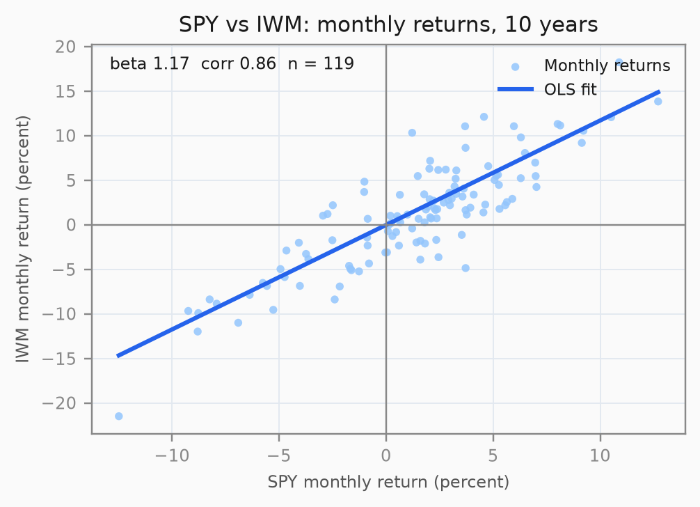
The sample numbers (as of 2026-08-20):
| Series | Mean (monthly) | Std dev (monthly) | Annualized mean | Annualized std |
|---|---|---|---|---|
| SPY | 1.30% | 4.44% | 16.8% | 15.4% |
| IWM | 1.03% | 6.04% | 13.1% | 20.9% |
| AGG (bond, for contrast) | 0.13% | 1.50% | 1.6% | 5.2% |
And the pair (covariance in decimal-return units): \(\text{Cov} = 0.002314\), \(\rho = 0.862\), \(\beta_{\text{IWM vs SPY}} = 1.173\), raw-return OLS intercept \(a_{\text{monthly}} = -0.49\%\).
Correlation 0.86 means the two equity funds usually move together (both are stocks), but not perfectly: the scatter's spread around the line is the residual noise. Beta 1.17 means a 1 percentage-point move in SPY relative to its fitted baseline is associated with about a 1.173 percentage-point move in IWM - small caps amplify market moves. The raw-return intercept of -0.49% per month is not CAPM excess-return alpha (that definition arrives in Unit 4), and a single window's intercept is exactly the kind of number Unit 5 teaches you not to over-trust. The bond fund (AGG) shows the contrast: low mean, low volatility, and - the point of the next lesson - low correlation with stocks, which is why bonds appear in every diversified portfolio.
The plot script and data fetch live at reference/investment-portfolio-theory/plots/. The numbers above were baked from the 2026-08-20 fetch; re-running fetch_data.py prints and saves a fresh summary, and the lesson text and plots must be regenerated separately from it (rule: live fetch, never commit price data - issue #6).
Systematic vs idiosyncratic risk (preview)
Write each asset's return as a market piece plus its own noise - the index model, which Unit 4 formalizes:
where \(r_m\) is the market return and \(e_i\) is the asset's firm-specific shock. The two conditions say the shock averages to zero and carries no systematic pattern with the market. Under this model the regression splits each asset's variance in a way Unit 4 formalizes:
Total risk = risk that follows the market (systematic, \(\beta^2\sigma_m^2\)) + risk specific to the asset (idiosyncratic, \(\sigma_e^2 = \text{Var}(e_i)\)). The equality holds because the shock is orthogonal to the market. The split matters because idiosyncratic risk can be diversified away by holding many assets - their noises cancel - while systematic risk cannot. In the scatter above, the vertical spread of points around the line is IWM's idiosyncratic risk.
Problem set
P1. Portfolio variance with covariance
SPY has \(\sigma = 15.4\%\), IWM has \(\sigma = 20.9\%\), and their correlation is 0.862 (annualized figures from the artifact). Compute the variance and standard deviation of a 50/50 portfolio.
Solution
\( \sigma_p^2 = 0.5^2(0.154)^2 + 0.5^2(0.209)^2 + 2(0.5)(0.5)(0.862)(0.154)(0.209) \).
\( = 0.25(0.023716) + 0.25(0.043681) + 0.5(0.027744) \)
\( = 0.005929 + 0.010920 + 0.013872 = 0.030721 \).
\( \sigma_p = \sqrt{0.030721} \approx 17.5\% \).
Check the story: the weighted average of the two volatilities is 18.15%, but the portfolio's volatility is 17.5% - lower than the average because correlation is below 1. The covariance term is what buys that reduction.
P2. Correlation from covariance
Two assets have \(\text{Cov}(r_1,r_2) = 0.002314\), \(\sigma_1 = 4.44\%\), \(\sigma_2 = 6.04\%\) (monthly). Compute the correlation. What would the correlation be if the covariance were -0.002314?
Solution
\( \rho = 0.002314 / (0.0444 \times 0.0604) = 0.002314 / 0.0026818 \approx 0.863 \).
If the covariance were -0.002314, the correlation would be -0.863: same magnitude, opposite sign. The normalization makes covariance comparable across assets; the sign carries the diversification message.
P3. Derive the covariance term in the n-asset sum
Show that for three assets, \(\text{Var}(r_p)\) with weights \(w_1, w_2, w_3\) equals \(\sum_i\sum_j w_i w_j \text{Cov}(r_i, r_j)\), by expanding \((w_1 d_1 + w_2 d_2 + w_3 d_3)^2\) and taking expectations. How many covariance terms appear?
Solution
Expanding the square: \(w_1^2 d_1^2 + w_2^2 d_2^2 + w_3^2 d_3^2 + 2w_1w_2 d_1d_2 + 2w_1w_3 d_1d_3 + 2w_2w_3 d_2d_3\).
Taking expectations: the squared terms become variances (3 of them), and each cross term \(2w_iw_j\text{Cov}(r_i,r_j)\) covers an unordered pair (3 of them). The double sum \(\sum_i\sum_j\) counts ordered pairs: 9 terms, of which 3 are variances (i=j) and 6 are covariances (each pair twice). For \(n\) assets: \(n\) variances and \(n(n-1)\) covariance contributions - the covariance terms dominate once \(n\) is at all large, which is lesson 0012's central fact.
P4. Derive beta from the OLS slope
Starting from the least-squares slope \(b = \sum \tilde{x}\tilde{y} / \sum \tilde{x}^2\), show that when \(x\) is the market return and \(y\) is an asset's return, \(b = \text{Cov}(r_i, r_m)/\text{Var}(r_m)\).
Solution
Divide numerator and denominator by \(n-1\):
\( b = \frac{\frac{1}{n-1}\sum \tilde{x}_t\tilde{y}_t}{\frac{1}{n-1}\sum \tilde{x}_t^2} = \frac{\text{Cov}(x,y)}{\text{Var}(x)} \).
With \(x = r_m\), \(y = r_i\): \( \beta = \text{Cov}(r_i, r_m)/\text{Var}(r_m) \). The sample estimates plug in exactly this way - which is why the scatter's OLS slope and the beta from the formula agree.
P5. Variance decomposition check
Using the artifact numbers: IWM's total variance is \(0.0604^2 = 0.003648\) (monthly). Its beta is 1.173 and SPY's variance is \(0.0444^2 = 0.001971\). Compute the systematic and idiosyncratic variance of IWM, and check they sum to the total.
Solution
Systematic: \( \beta^2\sigma_m^2 = 1.173^2 \times 0.001971 = 1.376 \times 0.001971 = 0.002712 \).
Idiosyncratic: \( 0.003648 - 0.002712 = 0.000936 \), i.e. \( \sigma_e = 3.06\% \) monthly.
So about 74% of IWM's variance is market-driven; 26% is its own noise. (These are sample numbers from one window - the decomposition logic is the lesson, not the exact percentages.)
P6. Interpret the artifact
Teach back, in plain language for a non-economist: what does "SPY and IWM have correlation 0.86 and beta 1.17" mean for someone deciding between holding only SPY, only IWM, or both?
Solution
A strong answer: correlation 0.86 means the two usually move in the same direction - both are stock markets - so splitting between them does not remove the market risk. But it is not 1, so the two funds are not the same bet: small caps (IWM) are a more aggressive version of the market (beta 1.17), swinging about 17% harder than SPY per unit of market move, plus their own extra noise.
Holding both instead of only SPY does two things: it keeps most of the market risk (the covariance term is large and positive) while adding some diversification against each fund's specific wobbles. The honest summary: for an investor who wants equity exposure, SPY + IWM is a diversification of style (large vs small), not a reduction of market risk - that reduction is what bonds (low correlation) or the risk-free asset buy, and that is lesson 0002's optimization question.
The two derivations (portfolio variance, OLS slope) are the unit's mastery targets. Re-derive them from scratch until you can do it without notes: the frontier (0013) and the CAPM (0016) are built on exactly these two results.