Utility, Risk Aversion, and Optimization
A score for every portfolio, and the two derivative moves that choose the best one.
Retrieve before reading
In one sentence: lesson 0001 left you with two assets and their covariance. What information is still missing before you can say how much to hold of each?
Reveal a strong answer
Your own preference for risk. The math tells you what combinations exist; it does not tell you which one you should pick. This lesson adds the missing ingredient: a utility score.
From moments to a score: the utility function
The course assumes each investor can attach a utility score to any portfolio, and uses the standard quadratic form (the one used in the CFA curriculum):
Read it in plain terms:
- \(E(r)\) is the reward - the bigger the better.
- \(\sigma^2\) is the risk - it subtracts from the score.
- \(A\) is the investor's risk aversion coefficient: how heavily risk is penalized. Higher \(A\) means more risk-averse.
- The \(1/2\) is a scaling convention; it makes the math come out cleanly in later derivations.
Utility is a score, not a return you receive. Two portfolios with the same score are equally attractive to this investor; the highest-score portfolio is the one they choose. The point of the function is that it converts the two-number summary (mean, variance) into a single ranking - and it ranks portfolios the way a risk-averse person actually does: penalizing variance, rewarding mean.
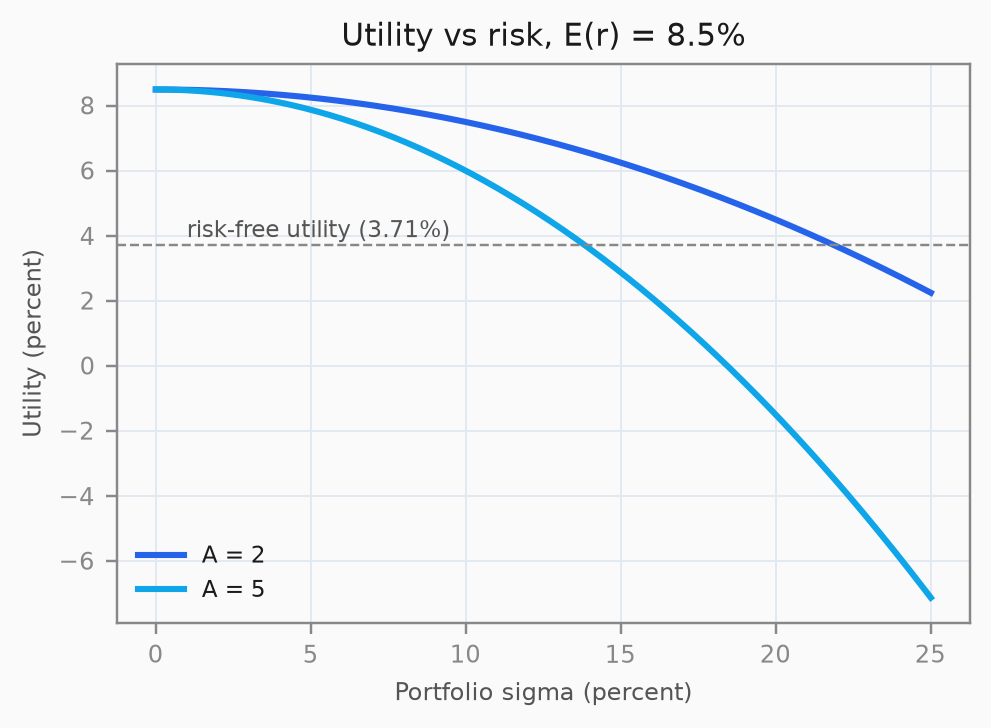
With \(E(r) = 8.5\%\) and the risk-free asset paying 3.71%: the risk-free asset has \(\sigma = 0\), so \(U_{rf} = 3.71\%\) for everyone. A risky portfolio with \(E(r) = 8.5\%\), \(\sigma = 20\%\) scores \(U = 8.5\% - 0.5A(0.04)\). For \(A = 2\): \(U = 8.5\% - 4\% = 4.5\%\), which beats the risk-free 3.71% - this investor does not hold 100% of this risky portfolio in preference to cash; as the optimization below shows, they hold about 60% of it. For \(A = 5\): \(U = 8.5\% - 10\% = -1.5\%\), worse than cash - this investor would not hold the portfolio all-in, and after optimizing holds about 24%. Same portfolio, two different verdicts: that is risk aversion at work.
Preview: indifference curves (lesson 0011)
Fixing \(U\) at a constant, the utility formula traces a curve in \((\sigma, E(r))\) space: every portfolio on it gives the same score. These are indifference curves, and higher curves are better. Lesson 0011 (MPT) uses them to pick the optimal complete portfolio. Here they are only a preview of the picture behind the score - this lesson uses the utility function directly in the two optimization mechanics below.
The utility function encodes a preference, not a fact. "Risk is bad, reward is good, and how bad depends on the person" is the entire content. Everything else in this lesson is mechanical: given the score, which portfolio maximizes it?
Optimization mechanics 1: max utility over the risky share
The first of the two unit mechanics: how much of your money goes into a risky asset with known \(E(r)\) and \(\sigma\), when the rest earns the risk-free rate \(r_f\).
The portfolio: weight \(y\) in the risky asset, \(1-y\) in cash. Its moments (from lessons 0000-0001):
Plug into utility:
Maximize by setting the first derivative to zero:
The optimal risky share: the risk premium in the numerator, risk aversion and variance in the denominator. The mechanics confirm the intuition from the curve plot: a higher premium raises \(y^*\), a higher \(A\) or higher \(\sigma^2\) lowers it.
Worked example. \(E(r) = 8.5\%\), \(\sigma = 20\%\), \(r_f = 3.71\%\), \(A = 2\):
This investor puts about 60% in the risky asset. With \(A = 5\): \(y^* = 0.0479/0.2 = 0.24\) - 24%, because the penalty is heavier. Note the second derivative \(U''(y) = -A\sigma^2 < 0\): the stationary point is a maximum, not a minimum. This \(y^*\) is the unconstrained optimum; with a long-only constraint \(0 \le y \le 1\), clip the solution to that interval.
The Sharpe ratio: the score that does not need A
Notice that \(y^*\) depends on the person (through \(A\)). Before knowing \(A\), the best we can say about a risky asset in isolation is its reward per unit of risk:
the Sharpe ratio (named for Bill Sharpe). It is the slope of the line from the risk-free asset to the risky portfolio in \((\sigma, E(r))\) space - the capital allocation line (CAL), which lesson 0011 treats fully. For a fixed risk-free asset and unrestricted mixing along each risky ray, the ray with the higher Sharpe ratio gives the higher maximum utility, so a steeper CAL is better for everyone. Sharpe alone does not rank arbitrary risky portfolios for every \(A\) - but it is why the capstone grades its tangency portfolio by Sharpe ratio.
Optimization mechanics 2: the minimum-variance weights
The second unit mechanic: for two risky assets, find the weights that minimize portfolio variance. From lesson 0001:
Minimize: set the derivative to zero. Using \(\text{Cov}_{12} = \rho\sigma_1\sigma_2\):
Solve for \(w\):
The minimum-variance portfolio is the least risky combination of the two assets - no utility function needed, purely a fact about the assets. The second derivative is \(2\sigma_1^2 + 2\sigma_2^2 - 4\text{Cov}_{12} = 2\,\text{Var}(r_1 - r_2) \ge 0\), strictly positive unless the two returns differ only by a constant, so this is a minimum.
Worked example. SPY and AGG (bond fund), annualized: \(\sigma_1 = 15.4\%\), \(\sigma_2 = 5.2\%\), and take \(\rho = 0\) as a first approximation (equities vs aggregate bonds are near-zero correlated):
About 10% in SPY, 90% in AGG. The low-volatility asset dominates the minimum-variance portfolio, and the covariance term only sharpens or softens the split depending on its sign.
Both unit mechanics are the same move: write the objective (utility or variance) as a function of a weight, differentiate, set to zero, check the second derivative. Unit 3 (0013-0014) does exactly this with more assets and a Lagrangian; the habit you build here is the entire method.
Real market artifact: the risk-free rate and the equity premium
From lesson 0001's artifact: SPY's annualized mean return was 16.8% and its annualized volatility 15.4%. The 3-month T-bill (FRED DTB3) pays 3.71% as of 2026-08-18.
The numbers for this lesson:
- SPY's risk premium: \(16.8\% - 3.71\% \approx 13.1\%\).
- SPY's Sharpe ratio: \(13.1\% / 15.4\% \approx 0.85\).
- Optimal SPY share for \(A = 2\): \(y^* = 0.131 / (2 \times 0.154^2) = 0.131/0.0474 \approx 2.76\) - above 1, meaning this investor would lever up (borrow at the risk-free rate to hold more than 100% SPY).
The last number is the honest lesson: with a 10-year window this hot, a mild risk aversion coefficient says "borrow and buy." That is a statement about this window's realized premium, not a forecast - Unit 6's equity premium puzzle and Unit 5's skepticism about extrapolating history are the correctives. The arithmetic of utility is window-independent; the inputs are not. (A long-only investor would clip these solutions above 100% to \(y^* = 1\).)
Utility gives you a decision rule; the two mechanics give you the two moves you will reuse everywhere: split with cash (capital allocation) and split between risky assets (minimum variance, then frontier). Lesson 0011 rebuilds both with full portfolio choice.
Mastery check - Unit 0 Toolkit
Mastery check - Unit 0
- [ ] Derive from first principles, without notes: two-asset portfolio variance from Var(aX + bY); the OLS slope from minimizing SSE
- [ ] Solve the unit's problem sets, worked solutions checked
- [ ] Interpret the SPY/IWM artifact and explain its economic meaning in plain language
If all three boxes are honest ticks, the toolkit is done: you can read a return, summarize risk, combine two assets, fit a beta, and choose a risky share. Unit 1 (Fixed Income) starts from the same toolkit with a new asset class: bonds, coupons, and the time value of money.
Problem set
P1. Utility of a risky portfolio
A portfolio has \(E(r) = 12\%\), \(\sigma = 25\%\). The risk-free rate is 3.71%. (a) Compute utility for \(A = 2\) and \(A = 6\). (b) For which \(A\) does the investor prefer the portfolio over cash?
Solution
(a) \( U = 0.12 - 0.5A(0.25)^2 = 0.12 - 0.5A(0.0625) = 0.12 - 0.03125A \).
\(A=2\): \(U = 0.12 - 0.0625 = 5.75\%\). \(A=6\): \(U = 0.12 - 0.1875 = -6.75\%\).
(b) Cash yields \(U = 3.71\%\). Prefer the portfolio when \(0.12 - 0.03125A > 0.0371\), i.e. \(A < 0.0829/0.03125 = 2.65\). So \(A=2\) holds it, \(A=6\) does not.
P2. Optimal risky share
Using the 0001 artifact numbers (SPY: \(E(r) = 16.8\%\), \(\sigma = 15.4\%\); \(r_f = 3.71\%\)): compute \(y^*\) for \(A = 4\) and interpret it in one sentence.
Solution
\( y^* = (0.168 - 0.0371)/(4 \times 0.154^2) = 0.1309/(4 \times 0.023716) = 0.1309/0.094864 \approx 1.38 \).
Interpretation: even a moderately risk-averse investor (\(A=4\)) would want 138% of wealth in SPY on this window's numbers, borrowing 38% at the risk-free rate. The premium was that large over the last decade - which is exactly why the lesson warns against treating a window's premium as a forecast.
P3. Minimum-variance weights, derived and computed
Two assets: \(\sigma_1 = 20\%\), \(\sigma_2 = 30\%\), \(\rho = 0.3\). (a) Derive \(w^*\) from \(\sigma_p^2(w)\) (show the derivative step). (b) Compute the minimum-variance weights.
Solution
(a) \(\sigma_p^2 = w^2\sigma_1^2 + (1-w)^2\sigma_2^2 + 2w(1-w)\rho\sigma_1\sigma_2\). Derivative:
\( \frac{d}{dw} = 2w\sigma_1^2 - 2(1-w)\sigma_2^2 + 2(1-2w)\rho\sigma_1\sigma_2 = 0 \).
Collecting \(w\): \( w(\sigma_1^2 + \sigma_2^2 - 2\rho\sigma_1\sigma_2) = \sigma_2^2 - \rho\sigma_1\sigma_2 \), hence \( w^* = (\sigma_2^2 - \rho\sigma_1\sigma_2)/(\sigma_1^2 + \sigma_2^2 - 2\rho\sigma_1\sigma_2) \).
(b) \(\text{Cov} = 0.3 \times 0.2 \times 0.3 = 0.018\). \( w^* = (0.09 - 0.018)/(0.04 + 0.09 - 0.036) = 0.072/0.094 \approx 0.766 \). So about 77% in asset 1, 23% in asset 2.
Sanity: the higher-volatility asset gets the smaller weight, and positive correlation pushes weight toward the less risky asset.
P4. Sharpe and the cash mix
A portfolio splits wealth between cash (risk-free, \(r_f\)) and a single risky asset with \(E(r)\) and \(\sigma\), with risky weight \(y\). Show algebraically that the portfolio's Sharpe ratio equals the risky asset's Sharpe ratio for every \(y\). What happens if you mix two risky assets instead?
Solution
\( E(r_p) - r_f = y(E(r) - r_f) \) and \( \sigma_p = y\sigma \), so \( S_p = (E(r_p) - r_f)/\sigma_p = (E(r) - r_f)/\sigma = S \), independent of \(y\). Adding cash scales risk and excess return by the same factor, so the reward-per-risk ratio is unchanged; this slope is the capital allocation line, which lesson 0011 treats fully.
Mixing two risky assets: the portfolio's Sharpe is generally not constant across combinations - it varies, which is why a unique tangency portfolio (the one maximizing it) exists. That is lesson 0014's and the capstone's object.
P5. Derive: max utility, second derivative check
Derive \(y^* = (E(r) - r_f)/(A\sigma^2)\) from \(U(y)\), and show explicitly that the second derivative is negative, so the stationary point is a maximum.
Solution
\(U(y) = r_f + y(E(r) - r_f) - \frac{1}{2}Ay^2\sigma^2\). First derivative: \(U'(y) = (E(r) - r_f) - Ay\sigma^2\). Setting to zero: \(y^* = (E(r) - r_f)/(A\sigma^2)\).
Second derivative: \(U''(y) = -A\sigma^2\). Since \(A > 0\) and \(\sigma^2 > 0\), \(U'' < 0\) everywhere - the function is globally concave and the stationary point is the unique maximum. Concavity is the mathematical face of risk aversion: utility rises with \(y\) at a decreasing rate, then falls.
P6. Interpret the artifact
Teach back, in plain language: what does "SPY's Sharpe ratio over the last ten years was about 0.85" mean for a non-economist, and what is the one warning you would add?
Solution
A strong answer: the Sharpe ratio says how much return you got per unit of risk you endured - roughly 0.85% of extra return for every 1% of volatility, after the risk-free rate. A higher Sharpe means the risk was "well paid." Over this window, stocks paid unusually well.
The warning: this is a description of one ten-year window, measured with hindsight. Sharpe ratios move with the window; the same calculation in other decades has been much lower, and the equity premium puzzle (Unit 6) is precisely that the historical average is hard to explain with calm risk aversion. Do not extrapolate one window's 0.85 into a forecast.
Unit 0 is the toolkit - everything later assumes you can do the two mechanics and read the two moments. If the mastery check is not honest yet, redo P4/P5 of lesson 0000 and P1/P3 of this lesson before moving to Unit 1.