Lesson 00 · Unit 0 Toolkit · Investment & Portfolio Theory

Returns and Risk: mean, variance, and the language of finance

Learn to say what a return is, how to summarize it, and why risk is measured as variance.

Retrieve before reading

In one sentence: if a stock costs $100, pays a $5 dividend, and is worth $110 at the end of the year, how much did you make?

Reveal a strong answer

You made 15%: the $5 dividend plus the $10 price gain, divided by the $100 you put in. That number is the holding period return.

What a return is

The holding period return (HPR) is the total gain from an investment over a period, as a fraction of what you paid:

\[ HPR = \frac{\text{Ending value} + \text{Income} - \text{Cost}}{\text{Cost}} \]

(0000.1)

For a stock: ending value is the price at the end, income is the dividend. For a bond: income is the coupon, and the price moves matter too. The return is a rate, not an amount: it scales with whatever you invested, which is why it can be compared across assets of very different sizes.

Returns are what investors care about, but the future return is unknown. Finance handles this by treating the return as a random variable and summarizing it with two numbers: expected return (where the center is) and variance (how spread out it is).

Expected return

If you can assign probabilities to a small number of outcomes (a scenario analysis), the expected return is the probability-weighted average. Here $p_s$ is the probability of scenario $s$, and $r_s$ is that scenario's return:

\[ E(r) = \sum_{s} p_s \cdot r_s \]

(0000.2)

Suppose a stock costs $100 and you judge three states of the world:

State	Probability	End price	Dividend	HPR
Boom	0.25	$130	$5	35%
Normal	0.50	$105	$5	10%
Recession	0.25	$70	$5	-25%

The HPRs: Boom $ (130+5-100)/100 = 35\% $, Normal $ 10\% $, Recession $ (70+5-100)/100 = -25\% $. So:

\[ E(r) = 0.25(35\%) + 0.50(10\%) + 0.25(-25\%) = 7.5\% \]

(0000.3)

Notice the probabilities sum to 1 and each HPR is weighted by its chance. The expected return is not any outcome you will actually see; it is the center of the distribution.

Variance and standard deviation: why risk is measured this way

Risk is the spread of possible outcomes around the expectation. The standard measure is variance: the expected squared deviation from the mean.

\[ \sigma^2 = \sum_{s} p_s \left(r_s - E(r)\right)^2 \qquad \sigma = \sqrt{\sigma^2} \]

(0000.4)

For the stock above:

\[ \sigma^2 = 0.25(0.35-0.075)^2 + 0.50(0.10-0.075)^2 + 0.25(-0.25-0.075)^2 = 0.0456 \]

(0000.5)

\[ \sigma = \sqrt{0.0456} \approx 21.4\% \]

(0000.6)

Two features make this the risk measure rather than an arbitrary choice:

It is measured in the same units as the return (percent), because of the square root. Variance alone is in percent-squared, which has no natural reading; the standard deviation does.
If returns are normally distributed, $\mu$ and $\sigma$ fully describe the distribution (here $\mu$ is shorthand for $E(r)$). That is a big deal: two numbers, and you know everything about the range of outcomes, including the probability of a loss of any given size. The whole course works in mean-variance space because of this fact. Real returns are not exactly normal (they have fatter tails), but the approximation is the industry workhorse.

Economic intuition

Risk is not "volatility is bad" in the abstract. Variance measures the chance that the return you get differs from the return you expected. Investors dislike that uncertainty, and the course's whole framework starts from this single preference.

Estimating from history

Scenario probabilities are subjective. The objective alternative: use past returns as a sample. Over $n$ historical periods,

\[ \bar{r} = \frac{1}{n}\sum_{t=1}^{n} r_t \qquad s^2 = \frac{1}{n-1}\sum_{t=1}^{n} (r_t - \bar{r})^2 \]

(0000.7)

The sample uses $n-1$ in the denominator (degrees of freedom) because the mean is estimated from the same data. This is the arithmetic mean; the geometric mean (compounding) appears in lesson 0003.

Here is what ten years of S&P 500 (SPY) daily returns actually look like:

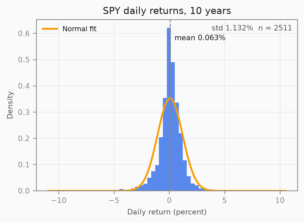
Histogram of SPY daily returns with a normal curve overlay — SPY daily returns, 2016-08-20 to 2026-08-20, Yahoo Finance (live fetch). [plot source]

Read the picture: the mean is about 0.063% per day, the standard deviation about 1.132% per day (2,511 trading days). The normal overlay fits the center well; the real distribution has fatter tails and a few outlier days. The daily numbers are small because a day is short; scaling them to a year (multiplying the mean by 252 trading days and the standard deviation by $\sqrt{252}$) gives about 15.9% and 18.0%. Note this is one annualization convention (daily arithmetic scaling) - lesson 0001 computes the same window from monthly returns with a compounding mean and a $\sqrt{12}$-scaled standard deviation, giving 16.8% and 15.4%. The two estimators agree in spirit, not exactly.

The risk-free rate, excess return, and the risk premium

Not all returns carry risk. A US Treasury bill is treated as essentially default-free, and its yield is the risk-free rate $r_f$. As of 2026-08-18, the 3-month T-bill (FRED series DTB3) pays 3.71%.

The excess return of an asset is $r - r_f$: what you earn beyond sitting in cash. The risk premium is the expected excess return:

\[ \text{Risk premium} = E(r) - r_f \]

(0000.8)

For the stock example above with $r_f = 3.71\%$: the risk premium is $7.5\% - 3.71\% = 3.79\%$. The economic question the premium answers: is 3.79% extra expected return enough compensation for a 21.4% standard deviation? That depends on risk aversion - the subject of lesson 0002.

Why this matters

Every later unit reuses these three building blocks: a return (HPR), its center (expected value), and its spread (variance). The Sharpe ratio, the frontier, the CAPM, and the capstone are all combinations of these ideas.

Problem set

P1. Compute an HPR

A bond is bought for $925.93. It pays a $60 coupon at year end and is sold for $950. What is the holding period return?

Solution

$ HPR = \frac{950 + 60 - 925.93}{925.93} = \frac{84.07}{925.93} \approx 9.08\% $.

The income (coupon) and the price gain both count; the return is relative to what you paid, not the face value.

P2. Expected return and variance from scenarios

A stock costs $50. Your scenario analysis: Boom (prob 0.20, end price $70, dividend $2), Normal (0.60, $55, $2), Recession (0.20, $40, $2). Compute the expected return and the standard deviation.

Solution

HPRs: Boom $(70+2-50)/50 = 44\%$, Normal $(55+2-50)/50 = 14\%$, Recession $(40+2-50)/50 = -16\%$.

$ E(r) = 0.20(0.44) + 0.60(0.14) + 0.20(-0.16) = 0.088 + 0.084 - 0.032 = 14.0\% $.

$ \sigma^2 = 0.20(0.44-0.14)^2 + 0.60(0.14-0.14)^2 + 0.20(-0.16-0.14)^2 = 0.20(0.09) + 0 + 0.20(0.09) = 0.036 $.

$ \sigma = \sqrt{0.036} \approx 18.97\% $.

P3. Moments from a small series

Five monthly returns: +2.0%, -1.0%, +3.5%, +0.5%, -2.5%. Estimate the mean and standard deviation (sample, $n-1$ denominator).

Solution

Mean: $(2.0 - 1.0 + 3.5 + 0.5 - 2.5)/5 = 2.5/5 = 0.5\%$.

Deviations: 1.5, -1.5, 3.0, 0.0, -3.0. Squares: 2.25, 2.25, 9.00, 0.00, 9.00. Sum: 22.50.

$ s^2 = 22.50/4 = 5.625\%^2 $, so $ s = \sqrt{5.625} \approx 2.37\% $.

The $n-1$ (not $n$) matters: with $n=5$ it raises the estimate from 4.50 to 5.625 percent-squared.

P4. Derive Var(aX)

From the definition of variance, show that $\text{Var}(aX) = a^2\text{Var}(X)$ for a constant $a$.

Solution

By definition, $\text{Var}(aX) = E\left[(aX - E[aX])^2\right]$.

Expectation is linear, so $E[aX] = aE[X]$. Then $aX - E[aX] = a(X - E[X])$, and

$ \text{Var}(aX) = E\left[a^2 (X - E[X])^2\right] = a^2 E\left[(X - E[X])^2\right] = a^2\text{Var}(X) $.

This is why scaling a position scales risk by the square of the scale - doubling the position quadruples the variance (and doubles the standard deviation). It is the seed of lesson 0001's portfolio variance formula.

P5. Linearity of expected return

A portfolio holds 60% in the stock of P2 and 40% in a risk-free asset paying 3.71%. Compute the portfolio's expected return two ways: (a) as the weighted average of the two expected returns, and (b) from first principles using $E[aX + bY] = aE[X] + bE[Y]$.

Solution

(a) $ E(r_p) = 0.60(14\%) + 0.40(3.71\%) = 8.4\% + 1.484\% = 9.884\% $.

(b) Linearity of expectation: for constants $a,b$ and random returns $X,Y$, $E[aX + bY] = aE[X] + bE[Y]$. With $a=0.60, b=0.40$, $X$ the stock return, $Y$ the risk-free return (a constant, so $E[Y]=Y$): same result, 9.884%.

The point of (b): the portfolio's expected return needs no assumption about correlation. Risk is where correlation shows up - lesson 0001.

P6. Interpret the artifact

Look at the SPY histogram. Explain, as if to a non-economist, what "mean 0.063% per day, standard deviation 1.132% per day" says about the market's reward and risk, and why a single bad day (-4% or worse) is rare but not impossible.

Solution

A strong answer covers three points:

Reward: on a typical day the market creeps up by about six hundredths of a percent. The daily mean annualizes to about 15.9% by simple scaling (about 17.2% if compounded) - that is a total return estimate. Subtracting the roughly 3.7% T-bill rate gives an excess return of roughly 12-13%, depending on the convention; that excess is the equity premium of this window.

Risk: the daily swings around that center are about 1.13% - most days land within about two standard deviations, i.e. roughly -2.2% to +2.3%. The size of the swing is the risk.

Tails: the histogram has more mass in the far tails than the normal curve predicts. A -4% day is a roughly 3.5-standard-deviation event under normality, but the real data shows it happened. That is the "fat tails" caveat: mean and variance describe the center well, but extreme days are more frequent than the normal model promises.

Do not rush

If P4 and P5 feel mechanical, that is fine - they are. They are the two algebraic habits (linearity of expectation, variance as expected squared deviation) that lesson 0001's derivations are built from.